Solving Bongard Problems With Deep Learning
Bongard problmes are named after their inventor, Soviet computer scientist Mikhail Bongard, who was working on pattern recognition in the 1960s. He designed 100 of this puzzles, to be a good benchmark for pattern recognition abilities, and they seem to be challenging for both people and algorithms. Here is an example:
 Figure 1.
Six images on the left conform to a rule, or a pattern, and the six images on the right conform to a different rule (usually an opposite). To solve the problem, one needs to understand the pattern and to figure out the rule (which is the solution). In this case, the rule is: “on the left: triangles, on the right: quadrilaterals”.
This one is easy, and it might take just few seconds to figure it out. But there are harder problems as well, for example:
 problem #22
 problem #29
 problem #37
 problem #54
You can test yourself by trying to find the rules. Solutions are here: 22, 29, 37, 54.
The problems became more well-known after appearing in the 1979 book “Gödel, Escher, Bach: An Eternal Golden Braid” by Douglas Hofstadter, who is himself a composer of Bongard problems [2]. Harry Foundalis, Hofstadter’s doctoral student, built an automated system to solve such problems as his Ph.D research project [3]. This system (called “Phaeco”) is not only a program for solving Bongard problems, but rather a cognitive architecture for visual pattern recognition.
Deep learning and Bongard problems
Results of Phaeco, created on 2006, are impressive. It is able to demonstrate solution of 15 problems (out of 280 collected by H.Foundalis), in many cases faster than people. It should be able to solve even more problems. But for this it would need additional extensive engineering for enhancement of features extractors/detectors [3].
Recently there has been significant advances in AI and ML, with deep neural networks winning numerous pattern recognition contests, and showing superhuman performance in some cases [4]. Fast implementations of convolutional neural networks (CNN) with max-pooling on GPUs has won large-scale ImageNet competition in 2012 [4], and in recent years there has been constant improvements in CNN algorithms and architectures.
So I could not help but wonder, if deep learning methods would be useful for solving Bongard problems. After trying to search for any information about it, I found only questions in online discussions:
“Deep learning” is the only interesting advance in AI since 1990.[…] I’m pretty sure deep learning would get nowhere with Bongard problems. I would be very surprised and impressed and excited if I were wrong! [https://meaningness.com/metablog/bongard-meta-rationality]
Anyone know if since then, say using deep learning or other newer methods, these problems are solvable easier? [https://news.ycombinator.com/item?id=12064188]
Bongard problems are inspiring some deep learning research [5]. But it is based on simplified images, with only few classes of generated images. Results are not conclusive for the original Bongard problems.
I decided to try to make a problems solver, something that I wanted to do since I learned about this problems in the first place.
Problem formulation and approach
There are at least two major problems with applying deep learning methods to Bongard problems.
1. it’s a one-shot learning problem. Most efficient applications of deep learning are based to supervised learning. For example, great results are shown for classifying image categories, after training on millions of images. In this case, neural networks show similar performance (or even better) that humans.
But in case of learning from only a few examples, in “one shot”, machine learning methods are nowhere near people in flexibility and performance [6]. BPs have only 6 examples for each class, and this is what makes them so hard for algorithms to solve.
2. It’s effectively a multi-modal learning problem. That is, input is in image form, and output is in the form of natural language description of classification rule. There are some approaches to solving such problems, but I did not have a clear idea for a solution. I decided to start with something simpler, with a goal of expanding to the full problem formulation later.
Instead of formulating the solution of a Bongard problem as a verbal description of a rule, it can be treated as a classification problem. In this case, 12 images are split into 2 groups: 10 “train” images and 2 “test” images. For train images, it’s knowns to which class they belong, left or right. Test images are swapped randomly, class for them is unknown.
Then, solving the problem would mean first looking at “train” images, and then deciding on a class assignment for test images.
Fig 3. shows how a problem is seen with this formulation.
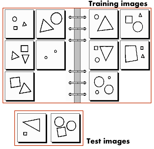 Figure 3.
Now, with simplified problem formulation, to actually solve it, I decided to apply transfer learning. It is one of the approaches to one-shot leaning which shows good results for visual analogy making [6, 7]. First, model is trained on many examples similar to target problem, and then relevant parameters from this model are reused.
Deep neural networks learn hierarchical feature representations of training data [8]. If a convolutional neural network is trained on Bongard images, it will learn features corresponding to different geometric shapes and their parts. Each feature can be thought of as a filter. If feature is present, certain layer and unit will be activated, which can be used by a classifier.
To train a feature extracting neural network (NN), it is not possible to to use images from BP. There are too few of them, only several hundreds, and they are too different to generalise to something meaningful. So I had to create a new dataset.
Synthetic dataset
For pre-training feature extracting neural network, I generated a set of random images, similar to images that occur in Bongard problems, which mainly contain geometrical primitives. Each image has one geometrical shape, with random position, scale, and rotation, If the shape is closed, it can be randomly filled with solid black color. In total there are 24 classes, descriptions and example images are shown below:
I generated 1M images for train set, and 10K for test set. Program for generating this images is on github: https://github.com/coolvision/random_shapes_generator
Neural network
To train a classifier of generated synthetic images, I used a relatively small neural network. It’s based on “Darknet Reference” model [9], with some maxpooling layers removed (because input image size is relatively small). It has 9 convolutional layers, architecture description shown below:
layer     filters    size              input                output
    0 conv     16  3 x 3 / 1   104 x 104 x   3   ->   104 x 104 x  16
    1 max          2 x 2 / 2   104 x 104 x  16   ->    52 x  52 x  16
    2 conv     32  3 x 3 / 1    52 x  52 x  16   ->    52 x  52 x  32
    3 conv     64  3 x 3 / 1    52 x  52 x  32   ->    52 x  52 x  64
    4 max          2 x 2 / 2    52 x  52 x  64   ->    26 x  26 x  64
    5 conv    128  3 x 3 / 1    26 x  26 x  64   ->    26 x  26 x 128
    6 conv    128  3 x 3 / 1    26 x  26 x 128   ->    26 x  26 x 128
    7 conv    128  3 x 3 / 1    26 x  26 x 128   ->    26 x  26 x 128
    8 conv    256  3 x 3 / 1    26 x  26 x 128   ->    26 x  26 x 256
    9 conv    512  3 x 3 / 1    26 x  26 x 256   ->    26 x  26 x 512
   10 conv     26  1 x 1 / 1    26 x  26 x 512   ->    26 x  26 x  26
   11 avg                       26 x  26 x  26   ->    26
   12 softmax                                          26
   13 cost
Figure 5. NN architecture
After training for 8 epochs, it converged to acceptable accuracy: top 1: 0.848000, top 2: 0.968000
Neural network output processing
First step in making a classifier for a Bongard problem is to put all 12 images through forward pass of a neural network. In convolutional neural networks, each layer has a set of filters with shared weights, and each filter’s response forms a feature map. Fig. 6 shows feature maps for all layers. Input image is on the left, and it is processed by successive layers, from left to right.
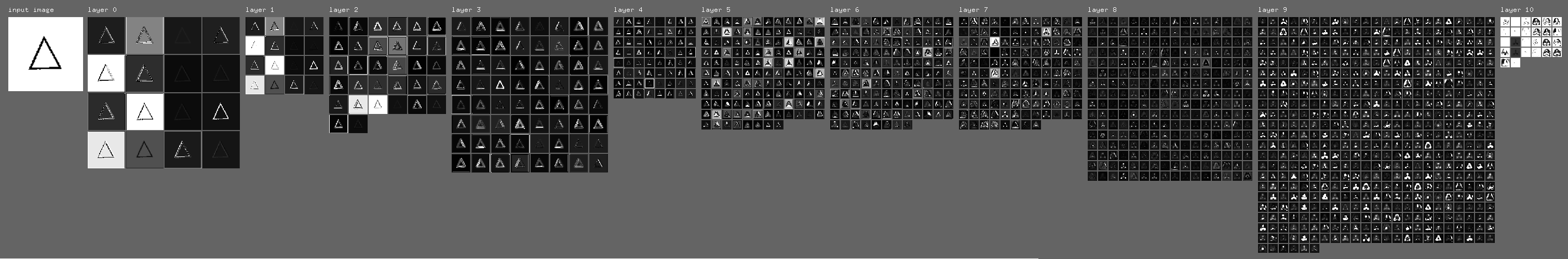
Figure 6. CNN feature maps (can be scrolled horizontally)
Each value (each “pixel”) in activation maps is potentially a feature. But values of this features are not invariant to positions, orientations, sizes, and other parameters of objects in input images. Classifier trained based on this features, on just 10 images, would not be be able to find an abstract classification rule, but would just quickly overfit.
To make features invariant to transformations, each feature map is transformed into a single binary feature in a following way: 1) normalize feature maps across layers, 2) threshold all values, with threshold set at 0.3 (Fig. 7), 2) if any value in a feature map is above threshold, set resulting feature to 1, otherwise to 0 (Fig. 8).
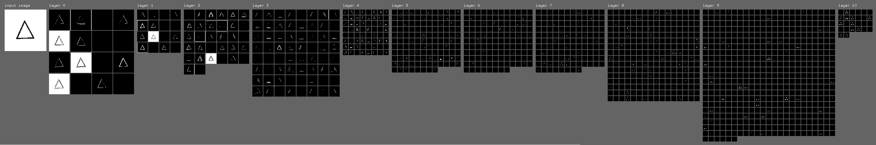
Figure 7. Feature maps after normalization and thresholding (can be scrolled horizontally).
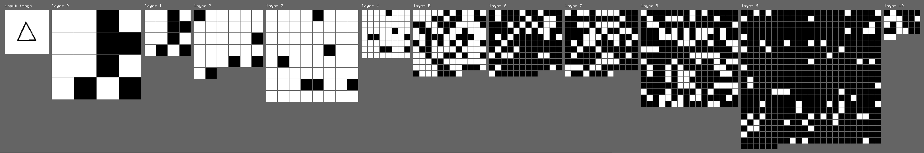
Figure 8. Binary features based on feature maps (can be scrolled horizontally).
This way, each image is described by CNN features. I ignored first several layers, and used only features from layers 6-10; There are 1050 feature maps in toatl on this layers, so each image is described with a binary vector of length 1050.
Finding classifier for problem solution
After features are extracted, they can be used for actually classifying problem images. I decided to use the simplest possible classifier, a decision stump (or 1-rule). It’s usually used as a part of more complex classifiers, but in this case might be sufficient. With this classifier, value of only one of the features is used to tell if image belongs to left or right group.
Algorithm for learning this rule is just a simple direct search. It can be demonstrated with an example of solving problem #6;
1) For 10 training images, features are extracted, as described above. For each image we have a binary feature vector, which describes this image (from NN point of view).
          f1 f2 f3 f4 f5 f6 f7  ... f1050
Image #1:  0  0  1  1  0  0  1  ... 0
Image #2:  1  0  1  0  0  1  0  ... 1
Image #3:  1  0  1  0  1  0  1  ... 0
Image #4:  0  0  1  0  1  1  0  ... 0
...
Image #10: 0  1  1  0  0  0  0  ... 1
Figure 9. Binary descriptors based on CNN features
2) For each feature, values for all 10 train images are checked. If values of the feature for 5 left images are different from values of features for 5 right images, it’s selected as possible classifier.
3) If several classifiers are found, we need a validation criterion to choose one of them. It’s possible to compare feature values for two test images: feature values should be different, because it’s a prior knowledge that they belong to different classes. Exact values of test classes ignored, only their equality is used as a validation criterion.
5) First classifier rule that passes validation is applied to test images, to check for correct classification. If it’s correct, problem is considered correctly solved.
6) If no rule was found, or no rule has passed validation, problem is considered unsolved.
Table 1 shows example of search for classification features for problem No 6 (shown on Figure 1). All features for which values on left and right images are different are shown. Only feature #731 passes validation, and after testing is found to be correct.
| Feature number | Values for train images | Values for test images | Validation status | Test status |
|---|---|---|---|---|
| 260 | 0 0 0 0 0 1 1 1 1 1 | 1 1 | False | - |
| 286 | 0 0 0 0 0 1 1 1 1 1 | 1 1 | False | - |
| 518 | 0 0 0 0 0 1 1 1 1 1 | 1 1 | False | - |
| 616 | 0 0 0 0 0 1 1 1 1 1 | 0 0 | False | - |
| 731 | 0 0 0 0 0 1 1 1 1 1 | 0 1 | True | True |
| 831 | 0 0 0 0 0 1 1 1 1 1 | 1 1 | False | - |
Table 1. Features analysis for problem #6.
Table 2 shows example of incorrectly classified problem #62. Two features were found to work as classifiers, both passed validation, but showed incorrect results for test images.
| Feature number | Values for train images | Values for test images | Validation status | Test status |
|---|---|---|---|---|
| 869 | 0 0 0 0 0 1 1 1 1 1 | 1 0 | True | False |
| 941 | 0 0 0 0 0 1 1 1 1 1 | 1 0 | True | False |
Table 2. Features analysis for problem #62.
The code for visualisations shown above, and for classification is on github: https://github.com/coolvision/bongard-problems-cnn
Results analysis
Results of running algorithm described above on 232 problems (from the list assembled by H. Foundalis), are following: solved: 47, correct: 41; That is, 20% of problems solved, with 87% accuracy.
To better show the results, solved problems are shown with color in Table 3, green — correct, and red — incorrect.
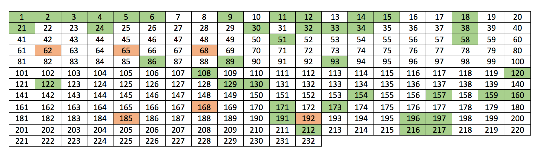 Table 3. Solved problems
Different parts of the problem set have different complexity, with first few dozens of problems being simpler. It is reflected in the results, Fig. 10 shows accuracy depending on problem number (computed for each consecutive group of 20 problems).
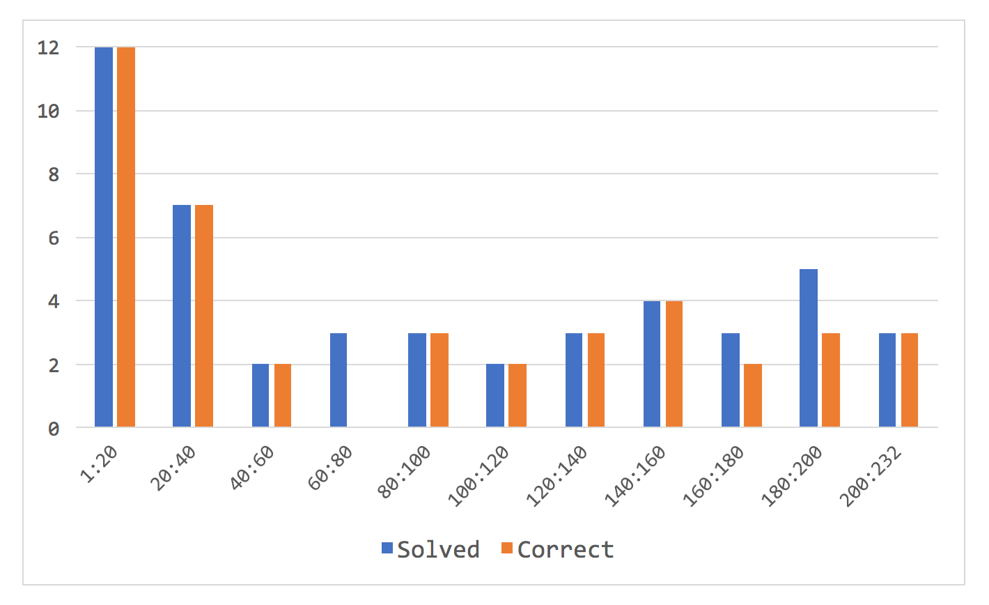 Figure 10. Solved problems accuracy, sorted by problem number
Table 4. shows accuracy for problems designed by different authors. First 100 problems, designed by M. Bongard, are the easiest to solve with my algorithm, and the rest are much more challenging.
| Author | Problem numbers | % solved | % correct |
|---|---|---|---|
| M.Bongard | 0-100 | 20 | 89 |
| D.Hofstadter | 100~156 | 10 | 100 |
| H.Foundalis | 157~200 | 25 | 73 |
| J.Insana | 200~232 | 10 | 100 |
Table 4. Average Accuracy for problems designed by different authors
In his thesis, H.Foundalis has collected data on people performance for solving problems #1-100. Fig. 11 shows accuracy of solving first 20. All problems are unique, and results vary a lot, but it shows that at least some of the problems are quite challenging even for people.
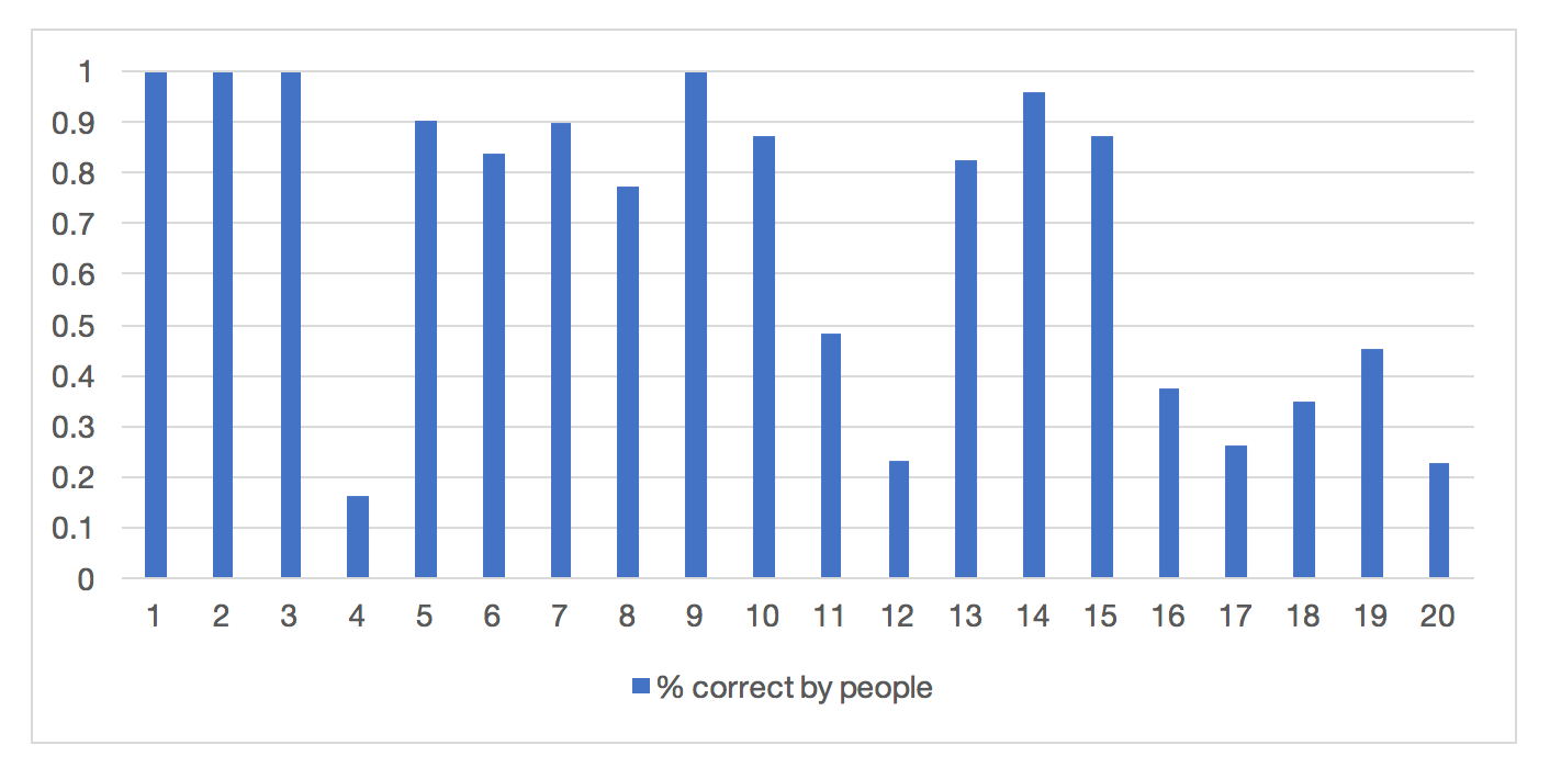 Figure 11. Accuracy of Bongard problems solutions by people
Conclusion
Simple off-the-shelf deep learning methods turned out to be useful for solving Bongard problems, at least in simplified classification form. It’s interesting that M. Bongard practically predicted something similar to approach described here, in “Pattern Recognition” [1]:
“…the purpose of the learning is not so much in finding a classifying rule (for example, a hyperplane), but rather in finding a feature space in which such separation is possible.”
In this case, feature space was created by pre-training of a neural network for classifying images similar to images in the problem domain.
“…after a “good” transformation of the image space into a feature space has already been found, there is practically no question of finding a classifying rule. It has been automatically found by that time.”
Original problem formulation includes explaining classification rules in natural language, which is fairly easy for people. It seems possible for “classical” algorithms based on hand-crafted features and patterns detectors (such as “Phaeco” [3]). But for neural networks, having transparent and explainable solutions is a known weak spot, so it might be more challenging. There are several ways to approach this:
-
Make a multi-modal synthetic dataset for supervised learning, including both images and rules explanations for Bongard problems. But, generating non-trivial puzzles is hard by itself, and even if it’s possible, I’m not sure that transfer learning would work in this case.
-
CNN visualization methods could be used to explain solutions. In this case, solution would be explained visually, with highlighting of pixels which were used for classification, and with showing what patterns are represented by CNN filters used for classification. It can be argued if visual explanation is as proper as verbal one, but to me it seems acceptable.
-
Generative NN architectures could be used as well, like variational autoencoder (VAE), or generative adversarial networks (GAN). In this case, it would be “explanation by example”.
“What I cannot create, I do not understand.”
― Richard FeynmanParaphrasing this quote, “What I can create, I understand”. NN would generate new examples of images from Bongard problems, and if this generated images capture the concepts behind classification rule, it might be enough to show understanding of the problem.
Overall, looks like even after 50 years, Bongard problems seem to still be a challenging benchmark for machine learning. It was a nice learning project, and I plan to continue working on a solver.
References
- Bongard, Mikhail M. (1970). Pattern Recognition. New York: Spartan Books.
- Hofstadter, D. R. (1979). Gödel, Escher, Bach: an Eternal Golden Braid. New York: Basic Books.
- Foundalis, H. (2006). Phaeaco: A Cognitive Architecture Inspired by Bongard’s Problems. Doctoral dissertation, Indiana University, Center for Research on Concepts and Cognition (CRCC), Bloomington, Indiana.
- Schmidhuber, J. (2015). Deep Learning in Neural Networks: An Overview. Neural Networks. 61: 85–117.
- Stabinger, Sebastian & Rodríguez-Sánchez, Antonio & Piater, Justus. (2016). Learning Abstract Classes using Deep Learning. Proceedings of the 9th EAI International Conference on Bio-inspired Information and Communications Technologies. 524-528.
- L. Fei-Fei, R. Fergus and P. Perona. (2006). One-Shot learning of object categories. IEEE Trans. Pattern Analysis and Machine Intelligence. Vol28(4): 594 - 611
- Liao, Jing & Yao, Yuan & Yuan, Lu & Hua, Gang & Bing Kang, Sing. (2017). Visual Attribute Transfer through Deep Image Analogy. ACM Transactions on Graphics. 36.
- Honglak Lee, Roger Grosse, Rajesh Ranganath, and Andrew Y. Ng. 2009. Convolutional deep belief networks for scalable unsupervised learning of hierarchical representations. In Proceedings of the 26th Annual International Conference on Machine Learning (ICML ‘09). ACM, New York, NY, USA, 609-616.
- Joseph Redmon. Darknet: Open Source Neural Networks in C. 2013–2016. http://pjreddie.com/darknet/